Definition

A stacked area chart is the extension of a basic area chart. It displays the evolution of the value of several groups on the same graphic. The values of each group are displayed on top of each other, what allows to check on the same figure the evolution of both the total of a numeric variable, and the importance of each group.

The following example shows the evolution of baby name frequencies in the US between 1880 and 2015.

# Libraries
library(tidyverse)
library(babynames)
library(streamgraph)
library(viridis)
library(hrbrthemes)
library(plotly)

# Load dataset from github
data <- babynames %>% 
  filter(name %in% c("Ashley", "Amanda", "Jessica",    "Patricia", "Linda", "Deborah",   "Dorothy", "Betty", "Helen")) %>%
  filter(sex=="F")

# Plot
p <- data %>% 
  ggplot( aes(x=year, y=n, fill=name, text=name)) +
    geom_area( ) +
    scale_fill_viridis(discrete = TRUE) +
    theme(legend.position="none") +
    ggtitle("Popularity of American names in the previous 30 years") +
    theme_ipsum() +
    theme(legend.position="none")
ggplotly(p, tooltip="text")

Note: This graphic does not have a legend since it is interactive. Hover a group to get its name. The dataset is available through the babynames R library and a .csv version is available on github.

What for

The efficiency of stacked area graph is discussed and it must be used with care. To put it in a nutshell:

stacked area graph are appropriate to study the evolution of the whole and the relative proportions of each group. Indeed, the top of the areas allows to visualize how the whole behaves, like for a classic area chart.
however they are not appropriate to study the evolution of each individual group: it is very hard to substract the height of other groups at each time point. For a more accurate but less attractive figure, consider a line chart or area chart using small multiple.

This website dedicates a whole page about stacking and its potential pitfalls, visit it to go further.

Variation

A variation of the stacked area graph is the percent stacked area graph. It is the same thing but value of each group are normalized at each time stamp. That allows to study the percentage of each group in the whole more efficiently:

p <- data %>% 
  # Compute the proportions:
  group_by(year) %>%
  mutate(freq = n / sum(n)) %>%
  ungroup() %>%
  
  # Plot
  ggplot( aes(x=year, y=freq, fill=name, color=name, text=name)) +
    geom_area(  ) +
    scale_fill_viridis(discrete = TRUE) +
    scale_color_viridis(discrete = TRUE) +
    theme(legend.position="none") +
    ggtitle("Popularity of American names in the previous 30 years") +
    theme_ipsum() +
    theme(legend.position="none")
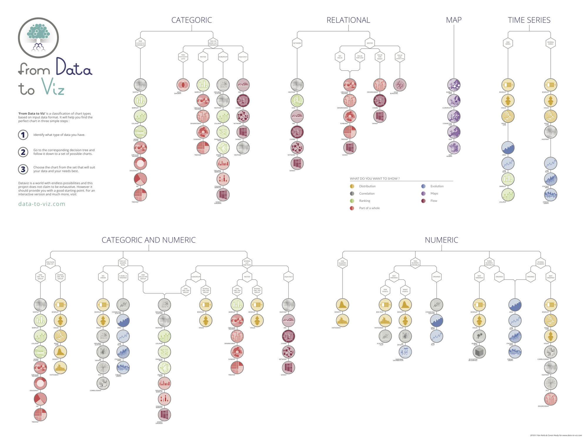
ggplotly(p, tooltip="text")

Common caveats

Use it with care, try using small multiple with area chart or line chart instead.
The group order (from bottom to top) can have an influence, try several orders.

Line plot

Displays the evolution of one or several numeric variables.

Area chart

Basically a line graph, filling the area under the curve.

Stacked area chart

Displays the evolution of the value of several groups on the same graphic

Streamgraph

A stacked area graph displaced around a central axis, resulting in a flowing, organic shape

Build your own

The R and Python graph galleries are 2 websites providing hundreds of chart example, always providing the reproducible code. Click the button below to see how to build the chart you need with your favorite programing language.

R graph gallery Python gallery

Comments

Any thoughts on this? Found any mistake? Disagree? Please drop me a word on twitter or in the comment section below: